Applications

Geometry module

Microstructure with equiaxed grains

Voronoi and Laguerre tessellations are some of the popular methods for generating polycrystalline microstructures. These approaches require positions and weights as input parameters for generating tessellation cells that resemble grains of a polycrystal. In this regard, the proposed particle packing approach can be used to generate the required information. Microstructures with equiaxed grains are best approximated by spheres, and after obtaining the necessary packing fraction, positions and radii can be outputted.

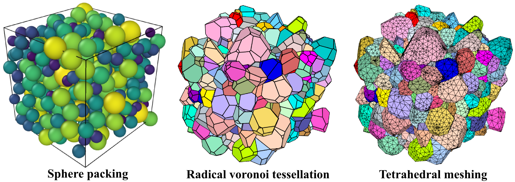
Figure: An example of sphere packing (left), radical Voronoi tesselation (center) and FE tetrahedral mesh (right).

In this example, to obtain a high packing fraction, the box size is set as the volume sum of all the spheres. This definition of the box size will inevitably result in an overlap of spheres at the final stages of the simulation. This is because the packing fraction of \(100\%\) is unachievable without the occurrence of overlaps. A reasonable amount of overlap is accepted, as the input data obtained from microstructure characterization techniques (like EBSD) are also approximations. Hence, for further post-processing, it is suggested to choose the time step at which the spheres are tightly packed and at which there is the least amount of overlap. The remaining empty spaces will get assigned to the closest sphere when it is sent to the tessellation and meshing routine. Complete freedom in selecting the desired time step of the simulation to be sent for further processing is one of the highlights of this approach.

Using the information obtained from sphere packing, radical Voronoi tessellation can be performed by Neper. And FE discretization of the tessellation cells by tetrahedral elements can also be done within Neper - Quey (2011) with assistance from the FE mesh generating software Gmsh - Geuzaine (2009).

Microstructure with elongated grains

Microstructures generated through conventional manufacturing processes like rolling and state-of-the-art processes like additive manufacturing (AM) consist of both elongated and equiaxed grains. In the context of AM, this is due to the complex solidification process, which occurs as a result of constant re-heating and re-cooling of previously melted layers during the manufacturing. The morphology of the grains along with the texture plays an important role in the resulting mechanical behavior. Hence, modeling such complex microstructures is vital, and in this regard the proposed approach of random ellipsoid packing is used.

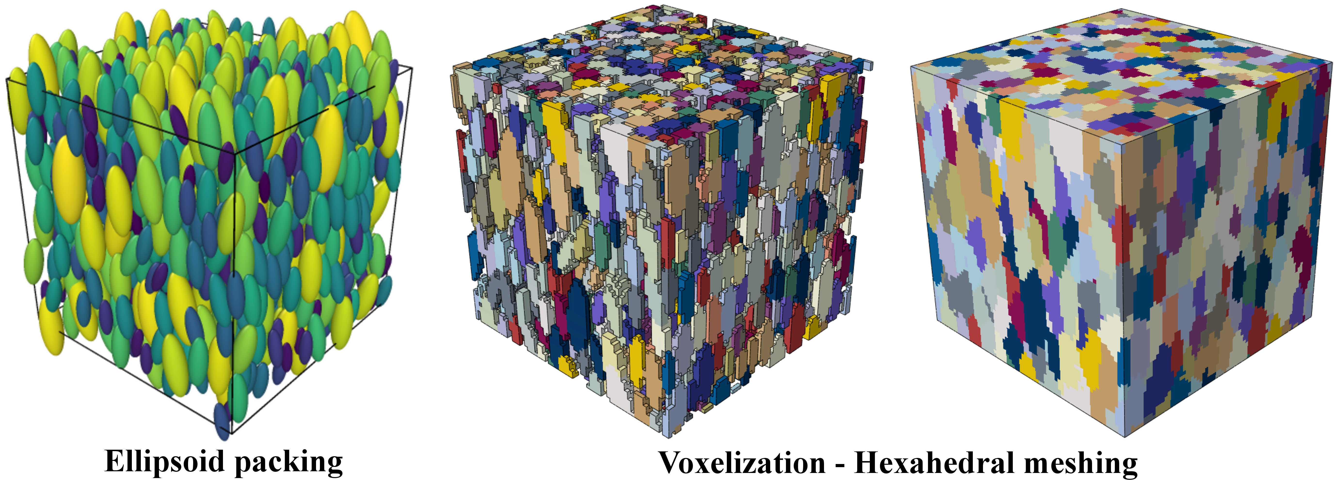
Figure: An example of ellipsoidal packing (left), Voxelization - FE hexahedral mesh (right).

The ellipsoid packing process is similar to that of sphere packing as described earlier. Once the ellipsoids are tightly packed with minimal acceptable overlaps, they are processed further for meshing. Since Voronoi tessellations cannot be applied to anisotropic particles such as ellipsoids, a voxel-based mesh-generating routine that utilizes convex hull for discretizing the RVE is employed. The voxelization (meshing) routine is made of 2 stages. The number of voxels in the RVE has a direct influence on the FE solution and the FE simulation time and must hence be meticulously chosen. The choice is not arbitrary, as it is constrained by how well the grains of the RVE are represented with respect to their geometry and the FEM simulation time.

Simulation benchmarks

To estimate the performance of Kanapy with respect to its particle packing and voxelization routines, multiple realizations of both sphere and ellipsoid packing was performed on a 2.60 GHz Intel Xeon CPU. Figure 1 depicts graphically the average CPU time recorded over 10 simulation runs for each realization of particle packing. The data is tabulated in Table 1. A significant difference in the variation of CPU time can be observed between spheres and ellipsoids of the same number. The difference arises from the fact that, two layered collision detection is sufficient to estimate if spheres collide. But ellipsoid collision detection requires an additional computational step of solving the characteristic equation as described in Overlap detection.

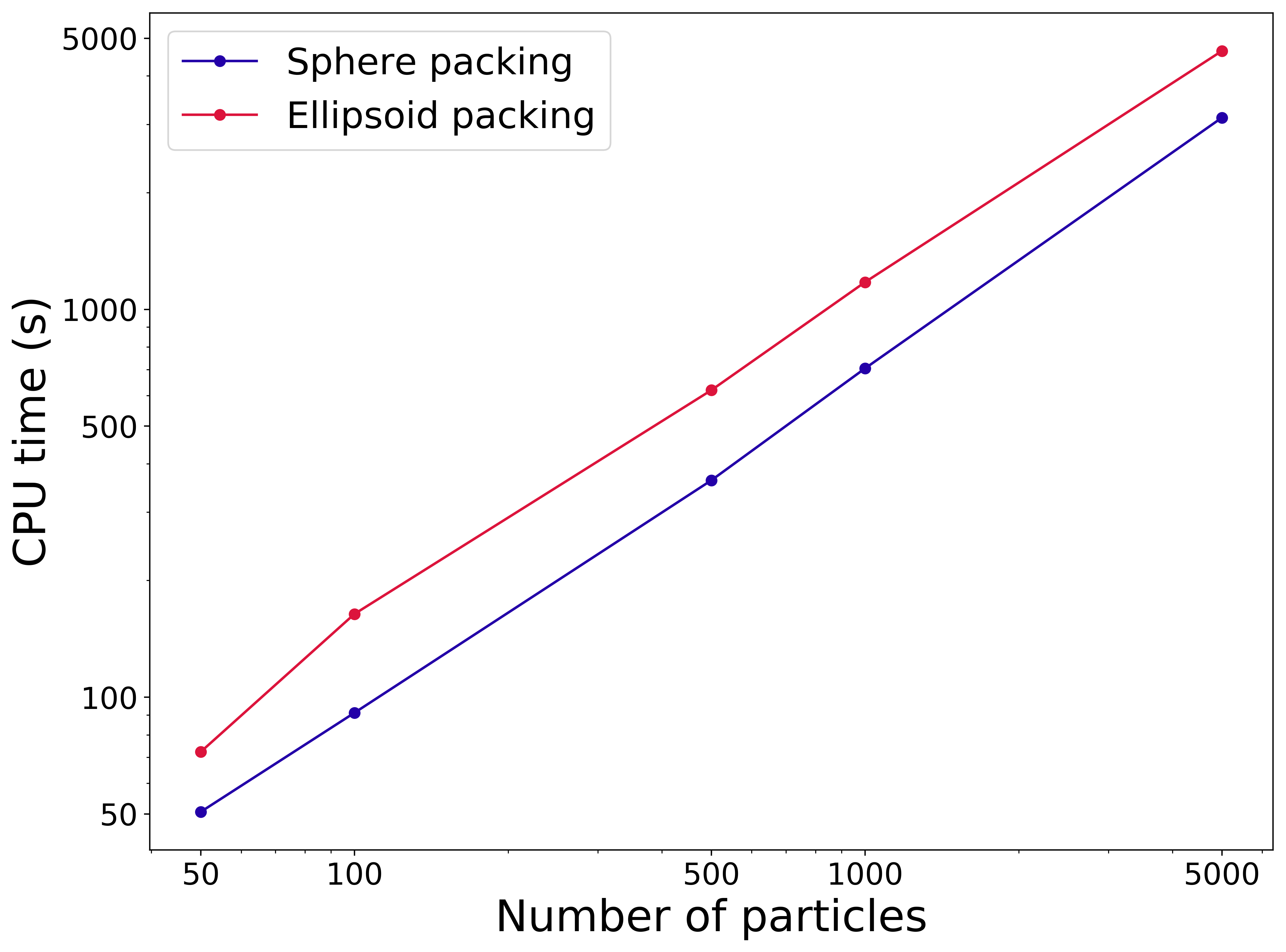
Figure 1: Log-log plot depicting the performance of the particle packing routine in terms of average CPU time (in seconds) recorded for different realizations of packing of spheres and ellipsoids.

Table 1: Particle packing simulation tests for spheres and ellipsoids. The CPU time is averaged over 10 simulation runs.

Number of	CPU time (s)
particles	Sphere	Ellipsoids
50	50.63	72.29
100	91.15	163.88
500	362.32	618.73
1000	704.13	1174.94
5000	3119.56	4635.41

Figure 2 depicts the CPU time recorded for the kanapy’s voxelization routine. The CPU time is estimated for various combinations of number of grains and number of voxels. These results are tabulated in Table 2.

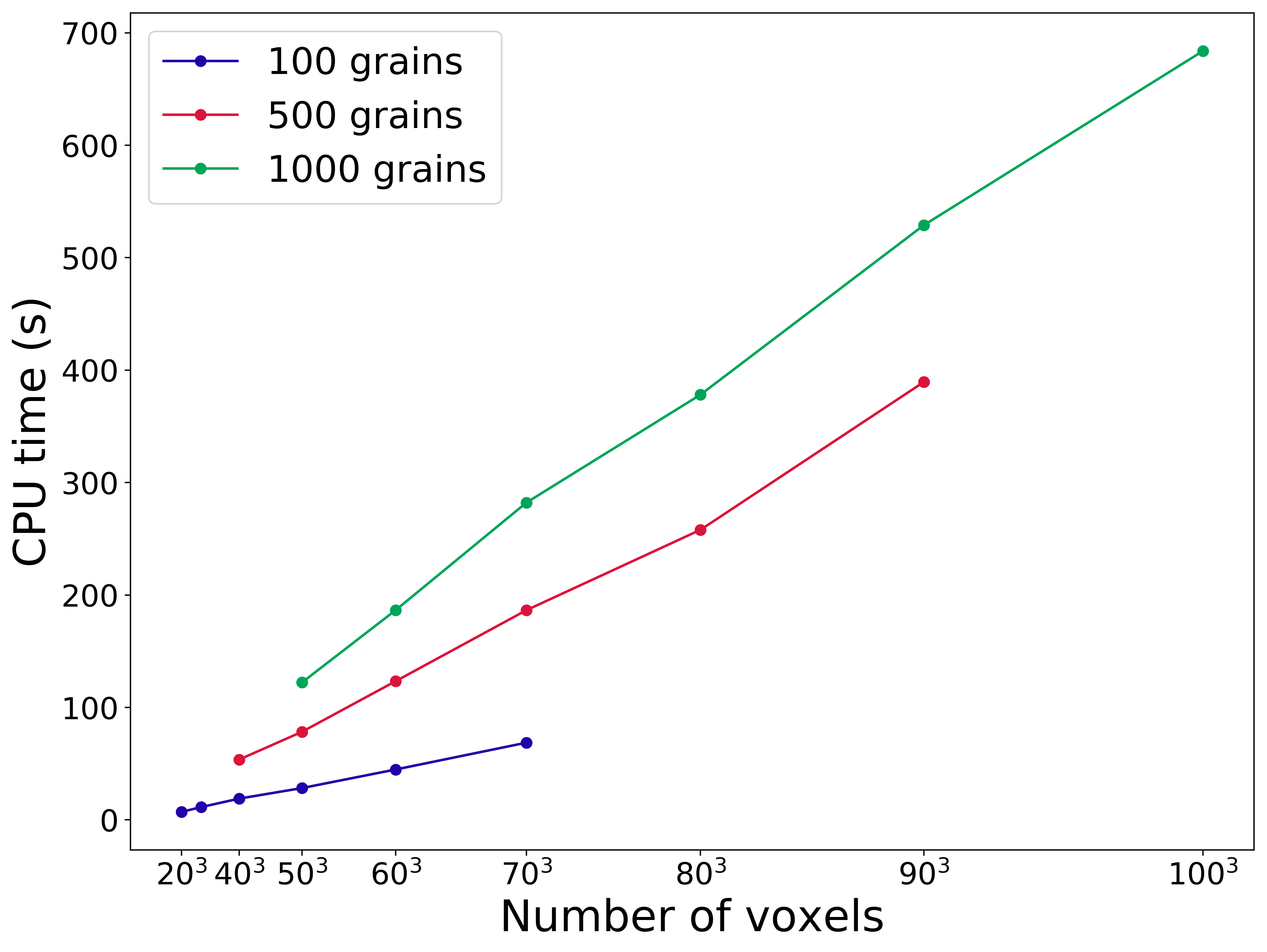
Figure 2: Plot depicting the performance of the voxelization routine in terms of CPU time (in seconds) for various combinations of grain numbers and total voxel numbers.

Table 2: Voxelization routine performance data for various combinations of grain numbers and total voxel numbers.

Number of voxels		CPU time (s)
	100 grains	500 grains	1000 grains
\(20^3\) = 8000	7.09
\(30^3\) = 27,000	11.33
\(40^3\) = 64,000	18.9	53.63
\(50^3\) = 125,000	28.26	78.33	122.19
\(60^3\) = 216,000	44.79	123.36	186.54
\(70^3\) = 343,000	68.65	186.49	282.17
\(80^3\) = 512,000		257.95	378.13
\(90^3\) = 729,000		389.48	528.95
\(100^3\) = 1,000,000			683.30

Texture module

The ODF reconstruction and the orientation assignment algorithms are both implemented as MATLAB functions within Kanapy. Both these algorithms utilizes several MTEX Bachmann (2010) functions, and are called within Kanapy by python. The ODF reconstruction algorithm can be used independently (if the required inputs are provided), whereas the orientation assignment algorithm only works if the ODF reconstruction is performed and the RVE is generated by Kanapy’s geometry module. The ODF reconstruction MATLAB function can also be used as a standalone program outside of Kanapy’s framework, but it still requires MTEX installation. Please refer to the comments in the MATLAB scripts for their independent usage. Various possible input configurations are discussed below, which have been exemplified using the Titanium EBSD data available within MTEX.

Since both these algorithms are implemented as MATLAB functions that calls other MTEX functions, the MATLAB and MTEX installation paths are required for Kanapy’s texture module. Make sure to set up the texture module within kanapy by running the command:

$ conda activate knpy
(knpy) $ kanapy setuptexture

ODF reconstruction

To use the ODF reconstruction algorithm, the EBSD data estimated using MTEX must be given as input in the form of (.mat) file. By providing the number of discrete orientations (\(N^\prime\)) required, the algorithm can be used in the minimum possible configuration. Note here the value of \(\kappa\) is set to a default value of \(0.0873\) rad. Figure 3 depicts the pole figure (plotted using MTEX) estimated from the experiment EBSD data file provided and Figure 4 depicts the pole figure for 250 discrete orientations obtained as output with the default \(\kappa\) value.

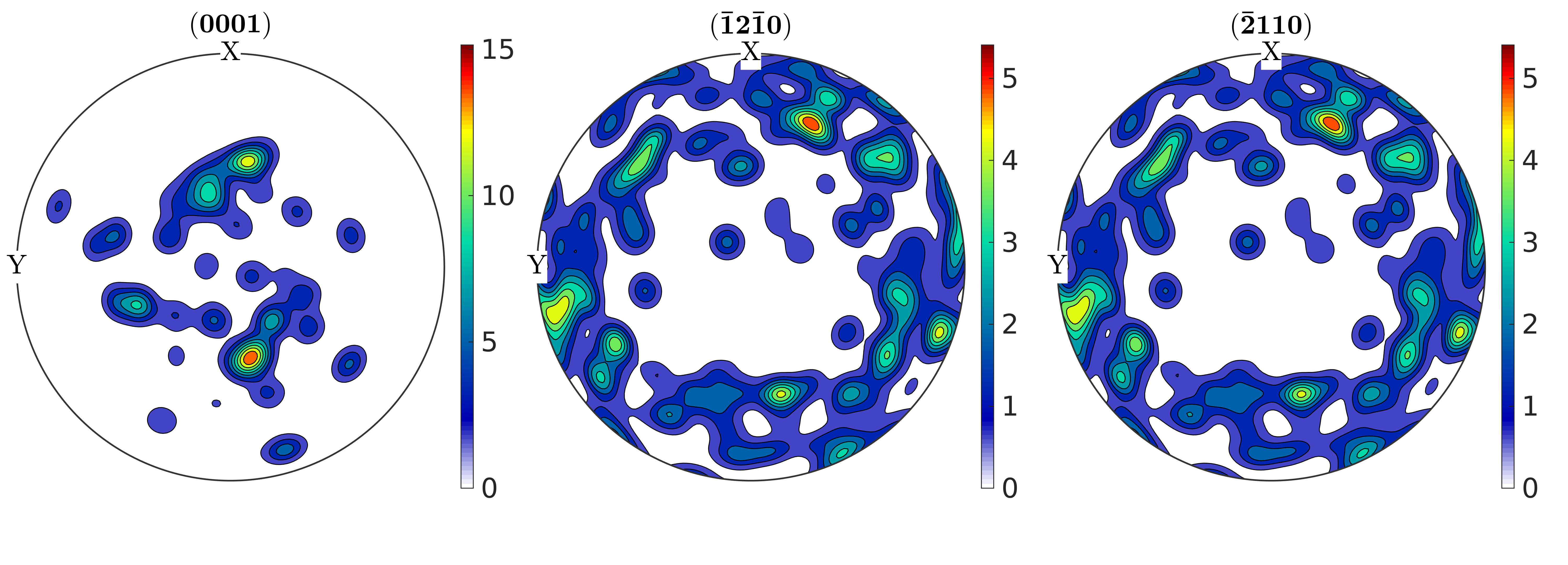
Figure 3: Plot depicting the pole figure obtained from EBSD data analysis.

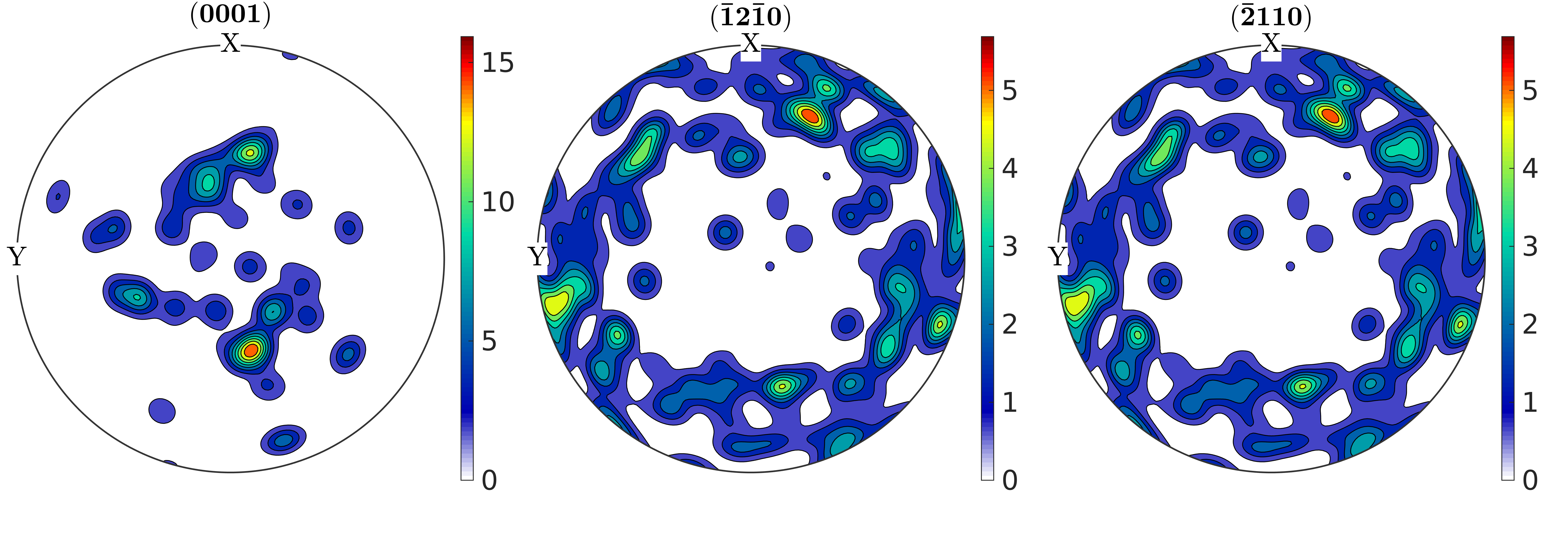
Figure 4: Plot depicting the pole figure obtained from 250 discrete orientation with default \(\kappa\) value of \(0.0873\) rad.

Alternately, the initial \(\kappa\) value can be specified (in radians) or the grains estimated using MTEX can be provided as an input in the (.mat) file format. If the grains (.mat) file is provided, then the optimum \(\kappa\) is estimated using the mean orientation of the grains (by an MTEX function). Figure 5 shows the pole figure (plotted using MTEX) estimated from EBSD data analysis and Figure 6 shows the pole figure for 250 discrete orientations obtained as output with \(\kappa\) value estimated using grain mean orientation.

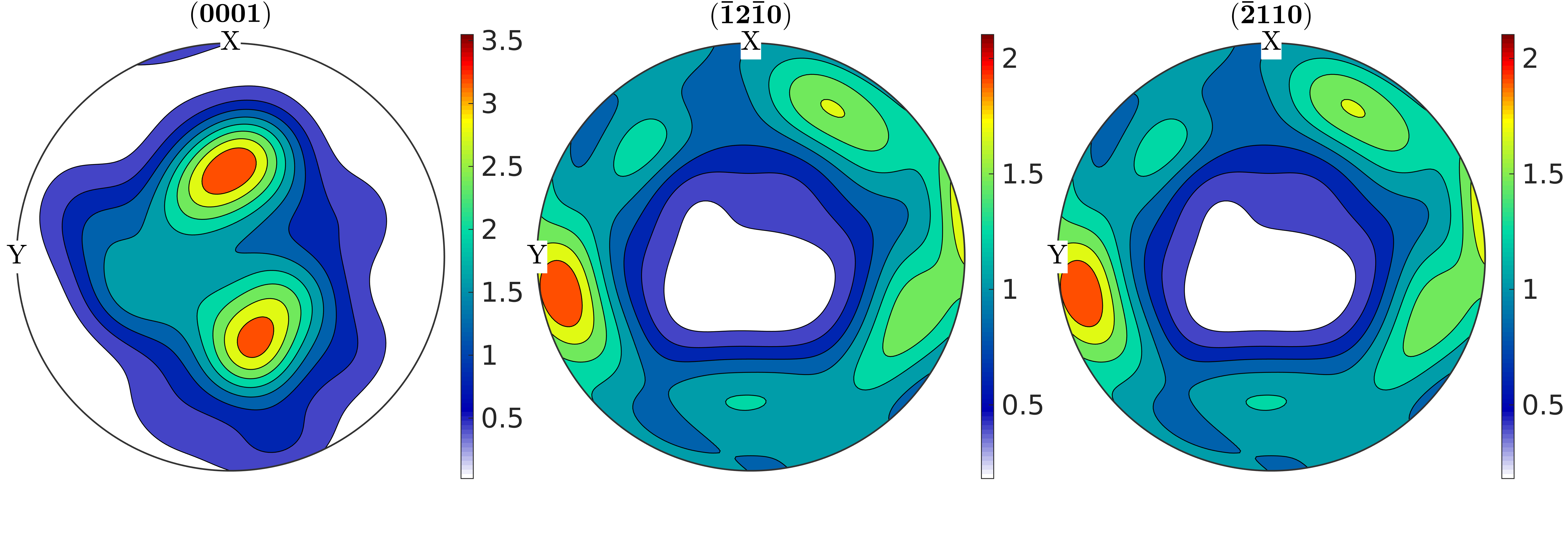
Figure 5: Plot depicting the pole figure of ODF data obtained from EBSD data analysis.

Figure 6: Plot depicting the pole figure of reconstructed ODF of 250 discrete orientation with \(\kappa\) value estimated using grain mean orientations.

The output from the ODF reconstruction algorithm is written to a (.txt) file, which consists of the \(L_1\) error of ODF reconstruction, the initial (\(\kappa\)) and the optimized (\(\kappa^\prime\)) values, and a list of the discrete orientations.

ODF reconstruction with orientation assignment

In addition to the ODF reconstruction, kanapy’s texture module can also be used to determine the optimal assignment of orientations to the grains. The orientation assignment algorithm can be used in this regard. The EBSD and the grain (.mat) files, along with the grain boundary shared surface area information are the required mandatory inputs. The grain boundary shared surface area is the output that is available after generating the RVE using kanapy’s geometry module. As explained earlier the surface area is used as weights for estimating the disorientation angle distribution.

An optional input that can be provided is the grain volume information, which is used for weighting the orientations after assignment and for estimating the ODF represented by the RVE. Figure 7 shows the ODF reconstructed using 250 discrete orientations weighted as per the grain volume (obtained from kanapy’s geometry module) and Figure 8 shows the comparison of the disorientation angle distribution between the EBSD data and the RVE (after orientation assignment).

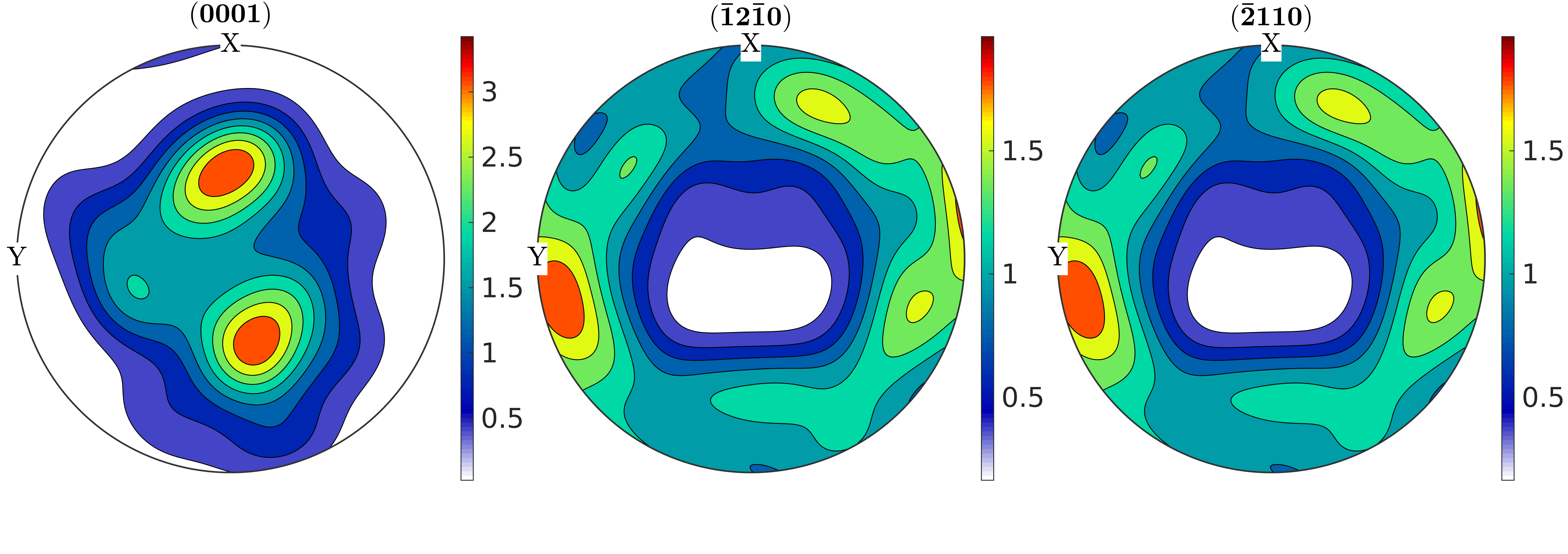
Figure 7: Pole figure of the ODF estimated after reconstruction with 250 discrete orientation weighted as per the grain volume and assigned using the orientation assignment algorithm.

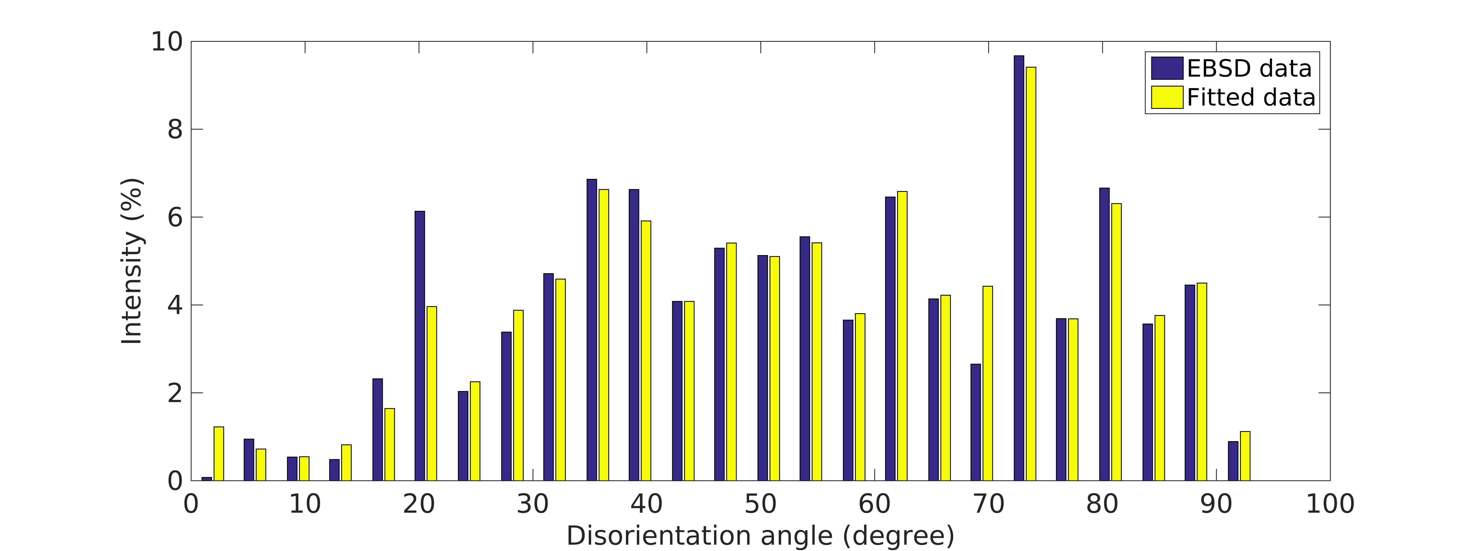
Figure 8: Bar plot depicting the comparison of the disorientation angle distribution between the EBSD data and the generated RVE.

The output of the orientation assignment algorithm is also written to a (.txt) file. It contains the \(L_1\) error due to ODF reconstruction, the \(L_1\) error between disorientation angle distributions from the EBSD data and the RVE, the initial (\(\kappa\)) and the optimized (\(\kappa^\prime\)) values, and a list of the discrete orientations each with a specific grain number that it should be assigned to.