Usage¶

Kanapy’s CLI¶

The available commands in Kanapy’s CLI and its usage is described here. The $ kanapy --help command details this as shown:

Note

Make sure that you are within the virtual environment created during the kanapy installation, as this environment contains the installed kanapy and its required dependencies.

$ conda activate knpy
(knpy) $ kanapy --help
        Usage: kanapy [OPTIONS] COMMAND [ARGS]...

        Options:
          --help  Show this message and exit.

        Commands:
          abaqusOutput  Writes out the Abaqus (.inp) file for the generated RVE.
          autoComplete  Kanapy bash auto completion.
          genDocs       Generates a HTML-based reference documentation.
          genRVE        Creates RVE based on the data provided in the input file.
          genStats      Generates particle statistics based on the data provided in...
          neperOutput   Writes out particle position and weights files required for...
          outputStats   Writes out the particle- and grain diameter attributes for...
          pack          Packs the particles into a simulation box.
          plotStats     Plots the particle- and grain diameter attributes for...
          readGrains    Generates particles based on the grain data provided in the...
          reduceODF     Texture reduction algorithm with optional Misorientation...
          runTests      Runs unittests built within kanapy.
          setupTexture  Stores the user provided MATLAB & MTEX paths for texture...
          voxelize      Generates the RVE by assigning voxels to grains.

The functionality and the arguments of each command listed above can be requested. For example:

(knpy) $ kanapy genStats --help
        Usage: kanapy genStats [OPTIONS]

          Generates particle statistics based on the data provided in the input
          file.

        Options:
          -f TEXT  Input statistics file name in the current directory.
          --help   Show this message and exit.

Note

Bash auto-completion option is avaiable for Kanapy’s CLI commands. Run: kanapy autoComplete to set it up

Detailed tutorial¶

Four examples come bundled along with the kanapy package. Each example describes a particular workflow that is either related to the geometry module or the texture module. Hence the examples are sub-categorized here under two sub-sections: Geometry examples and Texture examples. A detailed description of these examples is presented here. The two examples sphere_packing and ellipsoid_packing depict the different workflows that have to be setup for generating synthetic microstructures with equiaxed and elongated grains, respectively. And the two examples ODF_reconstruction and ODF_reconstruction_with_orientation_assignment depict the workflows for reconstructing ODF from EBSD data and assigning orientations to RVE grains, respectively. For a detailed understanding of the general framework of the packing simulations or the ODF reconstruction, please refer to: Modeling.

Note

New examples must be created in a separate directory. It allows the kanapy modules an easy access to the json, dump and other files created during the simulation.

Geometry examples¶

Both examples sphere_packing and ellipsoid_packing contain an input file wherein the user can specify the statistical parameters required for the simulation.

Note

The json and dump files help in making the various kanapy geometry modules independent of one another during execution.

Input file structure¶

An exemplary structure of the input file: stat_input.json is shown below:

{
  "Equivalent diameter":
    {
      "std": 0.39,
      "mean": 2.418,
      "cutoff_min": 8.0,
      "cutoff_max": 25.0
    },
  "Aspect ratio":
    {
      "std": 0.3,
      "mean": 0.918,
      "cutoff_min": 1.0,
      "cutoff_max": 4.0
    },
  "Tilt angle":
    {
      "std": 15.8774,
      "mean": 87.4178,
      "cutoff_min": 75.0,
      "cutoff_max": 105.0
    },
  "RVE":
    {
      "sideX": 85.9,
      "sideY": 112.33076,
      "sideZ": 85.9,
      "Nx": 65,
      "Ny": 85,
      "Nz": 65
    },
  "Simulation":
    {
      "periodicity": "True",
      "output_units": "mm"
    }
}

The input file is built in the JSON file format, with the following keywords: Equivalent diameter, Aspect ratio, Tilt angle, RVE, Simulation.

The keyword Equivalent diameter takes in four arguments to generate a log-normal distribution for the particle’s equivalent diameter; they are the Normal distribution’s standard deviation and mean, and the minimum and maximum cut-off values for the diameter. The values should correspond to $\mu m$ scale.

The Aspect ratio takes the mean and the standard deviation value value as input. If the resultant microstructure contains equiaxed grains then this field is not necessary.

The Tilt angle keyword represents the tilt angle of particles with respect to the positive x-axis. Hence, to generate a distribution, it takes in two arguments: the normal distribution’s mean and the standard deviation. If the resultant microstructure contains equiaxed grains then this field is also not necessary.

The RVE keyword takes two types of input: the side lengths of the final RVE required and the number of voxels per RVE side length.

The Simulation keyword takes in two inputs: A boolean value for periodicity (True/False) and the required unit scale ($mm$ or $\mu m$) for the output ABAQUS .inp file.

Note

The user may choose not to use the built-in voxelization (meshing) routine for meshing the final RVE. Nevertheless, a value for voxel_per_side has to be provided.
A good estimation for Nx, Ny & Nz value can be made by keeping the following point in mind: The smallest dimension of the smallest ellipsoid/sphere should contain at least 3 voxels.
The size of voxels should be the same along X, Y & Z directions (voxel_sizeX = voxel_sizeY = voxel_sizeZ). It is determined using: voxel size = RVE side length/Voxel per side.
Particles grow during the simulation. At the start of the simulation, all particles are initialized with null volume. At each time step, they grow in size by the value: diameter/1000. Therefore, the last timestep would naturally contain particles in their actual size.
The input unit scale should be in $\mu m$ and the user can choose between $mm$ or $\mu m$ as the unit scale in which output the ABAQUS .inp file will be written.

Workflows for sphere packing¶

This example demonstrates the workflow for generating synthetic microstructures with equiaxed grains. The principle involved in generating such microstructures are described in the sub-section Microstructure with equiaxed grains. With respect to the final RVE mesh, the user has the flexibility to choose between the in-built voxelization routine and external meshing softwares.

If external meshing is required, the positions and weights of the particles (spheres) after packing can be written out to be post-processed. The positions and weights can be read by the Voronoi tessellation and meshing software Neper for generating tessellations and FEM mesh. For more details refer to Neper’s documentation.

If the in-built voxelization routine is prefered, then kanapy will generate hexahedral element (C3D8) mesh that can be read by the commercial FEM software Abaqus. The Abaqus .inp file will be written out in either $mm$ or $\mu m$ scale.

$ conda activate knpy
(knpy) $ cd kanapy-master/examples/sphere_packing/
(knpy) $ kanapy genStats -f stat_input.json
(knpy) $ kanapy genRVE -f stat_input.json
(knpy) $ kanapy pack
(knpy) $ kanapy neperOutput -timestep 750

After navigating to the directory where the input file stat_input.json is located, kanapy’s CLI command genStats is executed along with its argument (name of the input file). It creates an exemplary ‘Input_distribution.png’ file depicting the Log-normal distribution corresponding to the input statistics defined in stat_input.json. Modifications can be made to the input statistics based on this plot. Next the genRVE command is executed to generate the necessary particle, RVE, and the simulation attributes, and it writes it to json files. Next the pack command is called to run the particle packing simulation. This command looks for the json files generated by genRVE and reads the files for extracting the information required for the packing simulation. At each time step of the packing simulation, kanapy will write out a dump file containing information of particle positions and other attributes. Finally, the neperOutput command (Optional) can be called to write out the position and weights files required for further post-processing. This function takes the specified timestep value as an input parameter and reads the corresponding, previously generated dump file. By extracting the particle’s position and dimensions, it creates the sphere_positions.txt & sphere_weights.txt files.

Note

The neperOutput command requires the simulation timestep as input. The choice of the timestep is very important. It is suggested to choose the time step at which the spheres are tightly packed and at which there is the least amount of overlap. The remaining empty spaces will get assigned to the closest sphere when it is sent to the tessellation and meshing routine. Please refer to Microstructure with equiaxed grains for more details.
The values of position and weights for Neper will be written in $\mu m$ scale only.

Note

For comparing the input and output statistics:

The json file particle_data.json in the directory ../json_files/ can be used to read the particle’s equivalent diameter as input statistics.
After tessellation, Neper can be used to generate the equivalent diameter for output statistics.

If the built-in voxelization is prefered, then the voxelize command can be called to generate the hexahedral mesh. It populates the simulation box with voxels and assigns the voxels to the respective particles (Spheres). The abaqusOutput command can be called to write out the Abaqus (.inp) input file. The workflow for this looks like:

$ conda activate knpy
(knpy) $ cd kanapy-master/examples/sphere_packing/
(knpy) $ kanapy genStats -f stat_input.json
(knpy) $ kanapy genRVE -f stat_input.json
(knpy) $ kanapy pack
(knpy) $ kanapy voxelize
(knpy) $ kanapy abaqusOutput
(knpy) $ kanapy outputStats
(knpy) $ kanapy plotStats

Note

The Abaqus (.inp) file will be written out in either $mm$ or $\mu m$ scale, depending on the user requirement specified in the input file.
For comparing the input and the output equivalent diameter statistics the outputStats command can be called. This command writes the diameter values in either $mm$ or $\mu m$ scale, depending on the user requirement specified in the input file.
The outputStats command also writes out the L1-error between the input and output diameter distributions.
The plotStats command outputs a figure comparing the input and output diameter distributions.

Storing information in json & dump files is effective in making the workflow stages independent of one another. But the sequence of the workflow is important, for example: Running the packing routine before the statistics generation is not advised as the packing routine would not have any input to work on. Both the json and the dump files are human readable, and hence they help the user debug the code in case of simulation problems. The dump files can be read by the visualization software OVITO; this provides the user a visual aid to understand the physics behind packing. For more information regarding visualization, refer to Visualize the packing simulation.

Workflows for ellipsoid packing¶

This example demonstrates the workflow for generating synthetic microstructures with elongated grains. The principle involved in generating such microstructures is described in the sub-section Microstructure with elongated grains. With respect to the final RVE mesh, the built-in voxelization routine has to be used due to the inavailability of anisotropic tessellation techniques. The Module voxelization will generate a hexahedral element (C3D8) mesh that can be read by the commercial FEM software Abaqus.

$ conda activate knpy
(knpy) $ cd kanapy-master/examples/ellipsoid_packing/
(knpy) $ kanapy genStats -f stat_input.json
(knpy) $ kanapy genRVE -f stat_input.json
(knpy) $ kanapy pack
(knpy) $ kanapy voxelize
(knpy) $ kanapy abaqusOutput
(knpy) $ kanapy outputStats
(knpy) $ kanapy plotStats

The workflow is similar to the one described earlier for sphere packing. The only difference being, that the neperOutput command is not applicable here. The outputStats command not only writes out the equivalent diameters, but also the major and minor diameters of the ellipsoidal particles and grains.

Note

A good estimation for the RVE side length values can be made by keeping the following point in mind: The biggest dimension of the biggest ellipsoid/sphere should fit within the corresponding RVE side length.
For comparing the input and output equivalent, major and minor diameter statistics, the command outputStats can be called. Kanapy writes the diameter values in either $mm$ or $\mu m$ scale, depending on the user requirement specified in the input file.
The outputStats command also writes out the L1-error between the input and output diameter distributions
The plotStats command outputs figures comparing the input and output diameter & aspect ratio distributions.

Texture examples¶

Both examples ODF_reconstruction and ODF_reconstruction_with_orientation_assignment require MATLAB & MTEX to be installed in your system. If your kanapy is not configured for texture analysis, please run the following command:

$ conda activate knpy
(knpy) $ kanapy setupTexture

Note

Your MATLAB version must be 2015 and above.
The required input files must be placed in the working directory from where the kanapy commands are run.

Workflow for ODF reconstruction¶

This example demonstrates the workflow for reconstructing ODF from experimental EBSD data. The principle involved in generating the reduced ODF is described in the sub-section ODF reconstruction. Kanapy requires the EBSD data estimated using MTEX as input in the (.mat) file format. In this regard, an exemplary EBSD file (titanium.mat) is provided in the ../kanapy-master/examples/ODF_reconstruction/ folder.

$ conda activate knpy
(knpy) $ cd kanapy-master/examples/ODF_reconstruction/
(knpy) $ kanapy reduceODF -ebsd titanium.mat

After navigating to the directory where the input file titanium.mat is located, kanapy’s CLI command reduceODF is executed along with its argument (name of the EBSD (.mat) file). If kanapy’s geometry module is executed already, then the number of reduced orientations are read directly. Else kanapy requests the user to provide the number of reduced orientations required before calling the MATLAB ODF reconstruction algorithm.

Note

The EBSD (.mat) file is a mandatory requirement for the ODF reconstruction algorithm.
Note here the value of the kernel shape parameter ($\kappa$) is set to a default value of 0.0873 rad.

Alternatly, an initial kernel shape parameter ($\kappa$) can be specified as an user input (OR) the grains estimated using MTEX can be provided as an input in the (.mat) file format. The value of $\kappa$ must be in radians, if user specified. Else if the grains (.mat) file is provided, then the optimum $\kappa$ is estimated by kanapy using the mean orientation of the grains. In this regard, an exemplary grains file (titanium_grains.mat) is provided in the ../kanapy-master/examples/ODF_reconstruction/ folder. The workflow for this looks like:

$ conda activate knpy
(knpy) $ cd kanapy-master/examples/ODF_reconstruction/
(knpy) $ kanapy reduceODF -ebsd titanium.mat -kernel 0.096
                                 (OR)
(knpy) $ kanapy reduceODF -ebsd titanium.mat -grains titanium_grains.mat

Note

The output files are saved to the /mat_files folder under the current working directory.
The output (.txt) file contains the following information: $L_1$ error of ODF reconstruction, the initial ($\kappa$) and the optimized ($\kappa^\prime$) values, and a list of discrete orientations.
Additionaly kanapy saves the reduced ODF and the reduced orientations (.mat) files in this folder.
Kanapy writes a log file (kanapyTexture.log) in the current working directory for possible errors and warnings debugging.

Workflow for ODF reconstruction with orientation assignment¶

This example demonstrates the workflow for reconstructing ODF from experimental EBSD data and then determining the optimal assignment of orientations to RVE grains. The principle involved in optimal orientation assignment is described in the sub-section ODF reconstruction with orientation assignment. In addition to the EBSD data, Kanapy requires grain (.mat) file, and the grain boundary shared surface area information as input. In this regard, an exemplary EBSD file (titanium.mat), and a grains file (titanium_grains.mat) are provided in the ../kanapy-master/examples/ODF_reconstruction_with_orientation_assignment/ folder. It is important to note that the grain boundary shared surface area file is created whilst generating an RVE by kanapy’s geometry module.

$ conda activate knpy
(knpy) $ cd kanapy-master/examples/ODF_reconstruction_orientation_assignment/
(knpy) $ kanapy genStats -f stat_input.json
(knpy) $ kanapy genRVE -f stat_input.json
(knpy) $ kanapy pack
(knpy) $ kanapy voxelize
(knpy) $ kanapy outputStats
(knpy) $ kanapy reduceODF -ebsd titanium.mat -grains titanium_grains.mat -fit_mad yes

After navigating to the directory where the input file titanium.mat is located, generate an RVE by calling kanapy’s geometry CLI commands: genStats, genRVE, pack & voxelize. To generate the shared surface area file, run outputStats command. Kanapy will write a shared_surfaceArea.csv file to the /json_files/ folder. This file contains the grain boundary shared surface area information between neighbouring grains. Now, kanapy’s texture CLI command reduceODF can be called along with its arguments (name of the EBSD, grains (.mat) files). The key -fit_mad must be used with this command to tell kanapy that orientation assignment to grains is required. Since kanapy’s geometry module is executed already, kanapy recognizes the number of reduced orientations required (=number of grains in the RVE). Else kanapy requests the user to provide the number of reduced orientations required before calling the MATLAB functions.

Note

The EBSD, grains (.mat) files and the grain boundary shared surface file are mandatory requirements for the orientation assignment algorithm.
The shared_surfaceArea.csv file is generated by running kanapy outputStats.

Additionally an optional input that can be provided is the grain volume information, which is used for weighting the orientations after assignment and for estimating the ODF represented by the RVE. Kanapy also writes the grains volume file (grainsVolumes.csv) to the /json_files/ folder, when the outputStats command is executed after RVE generation.

Note

The grainsVolumes.csv file lists the volume of each grain in the ascending order of the grain ID.
Kanapy automatically detects the presence of the shared_surfaceArea.csv & grainsVolumes.csv files, if they are present in the /json_files/ folder.
The output files are saved to the /mat_files folder under the current working directory.
The output (.txt) file contains the following information: $L_1$ error of ODF reconstruction, $L_1$ error between disorientation angle distributions from the EBSD data and the RVE, the initial ($\kappa$) and the optimized ($\kappa^\prime$) values, and a list of discrete orientations each with a specific grain number that it should be assigned to.
Additionaly kanapy saves the reduced ODF and the reduced orientations (.mat) files in this folder.
Kanapy writes a log file (kanapyTexture.log) in the current working directory for possible errors and warnings debugging.

Visualize the packing simulation¶

You can view the data generated by the simulation (after the simulation is complete or during the simulation) by launching OVITO and reading in the dump files generated by kanapy from the ../sphere_packing/dump_files/ directory. The dump file is generated at each timestep of the particle packing simulation. It contains the timestep, the number of particles, the simulation box dimensions and the particle’s attributes such as its ID, position (x, y, z), axes lengths (a, b, c) and tilt angle (Quaternion format - X, Y, Z, W). The OVITO user interface when loaded, should look similar to this:

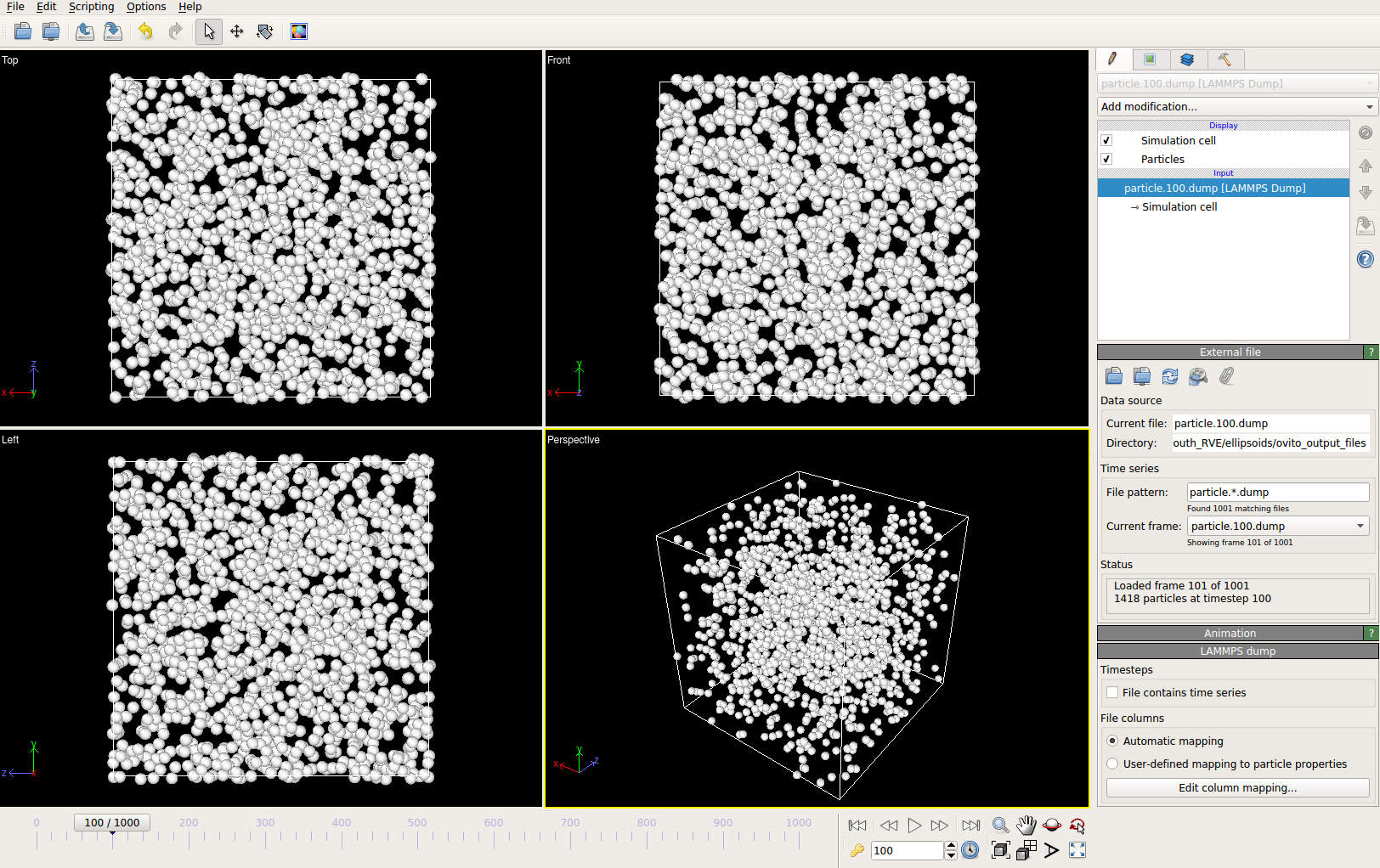
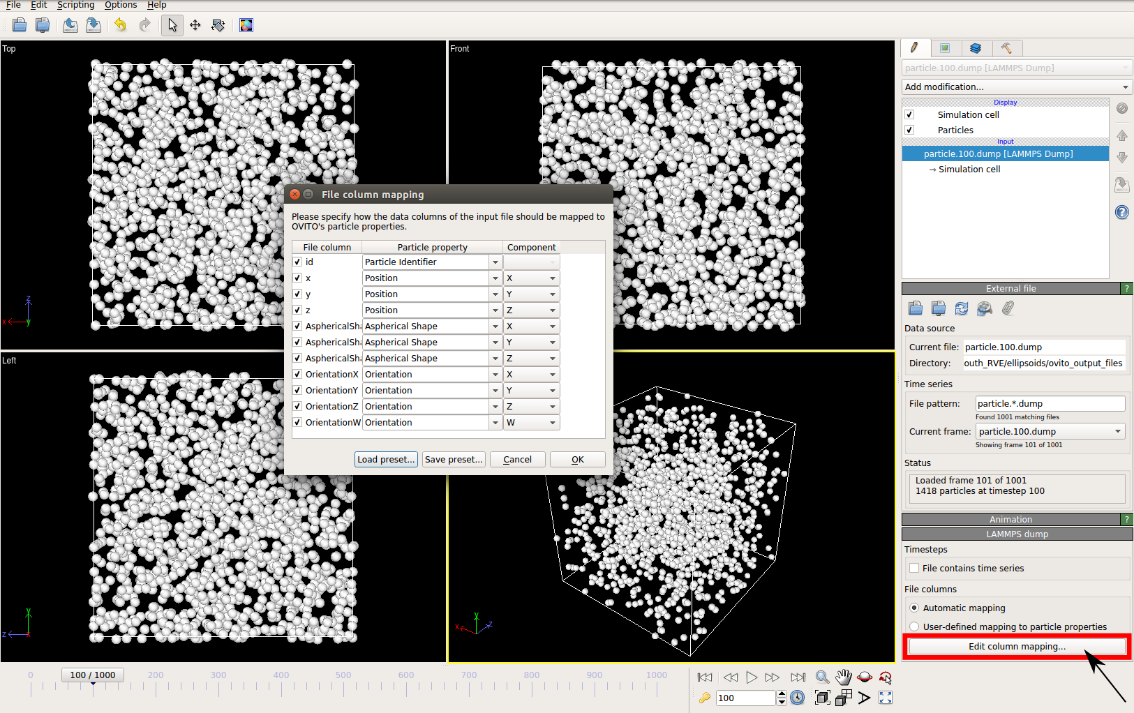
By default, OVITO loads the particles as spheres, this option can be changed to visualize ellipsoids. The asphericalshapex, asphericalshapey, and asphericalshapez columns need to be mapped to Aspherical Shape.X, Aspherical Shape.Y, and Aspherical Shape.Z properties of OVITO when importing the dump file. Similarily, the orientationx, orientationy, orientationz, and orientationw particle properties need to be mapped to the Orientation.X, Orientation.Y, Orientation.Z, and Orientation.W. OVITO cannot set up this mapping automatically, you have to do it manually by using the Edit column mapping button (at the bottom-right corner of the GUI) in the file import panel after loading the dump files. The required assignment and components are shown here:

For further viewing customizations refer to OVITO’s documentation.